How Macroeconomic Variables Impact Sector Performance
- Research shows that macroeconomic variables can impact some sectors differently than others.
- Inflation, gross domestic product, monetary and fiscal policy can all affect asset prices.
- While there are many variables that impact asset prices, investors should not ignore macro factors.
Macroeconomic variables like inflation, monetary policy, GDP growth, and commodity prices are important in explaining asset class performance and style premia — academic studies confirm it. The more directly the macroeconomic environment or specific economic variables affect a sector’s operating environment and financial results, the greater the impact on that sector’s performance. For example, oil prices directly affect the revenue, profitability, and asset value of Oil & Gas Explorers and Producers. And, interest rates movements are one of key drivers of Banks’ net interest margins.1
The goal of our research here is to identify sectors and industries that have greater performance sensitivity to specific macroeconomic variables. This gives investors a starting point for the kind of top-down sector analysis that can help guide investment decisions.
Identifying the Sector Opportunity Set
Certain sub-sectors or industries may exhibit greater sensitivity to macroeconomic variables than the broad sector. Our analysis of the 11 GICS sectors and 18 industries (see Appendix I) identifies this specific opportunity set for investors.
We focused on a few key indicators broadly recognized to be influencers of asset class performance, as shown in Figure 1. Then, we selected sample time periods based on the availability of historical sector performance data (starting from July 2003) or the full cycle of yield changes.
Figure 1: Macroeconomic Variables
| Macroeconomic Variables | Time Period |
|---|---|
| 10-Year Treasury Yield (%, Level Change) | January 2018 – December 2022, which is a full cycle of 10-year decline from 3% and rebound to 4% |
| 10-Year Breakeven Rate (Proxy for Inflation Expectation, %, Level Change) | July 2003 – December 2022 |
| US Dollar Index (%, Price Change) | July 2003 – December 2022 |
| WTI Crude Oil Prices (%, Price Change) | July 2003 – December 2022 |
Source: State Street Global Advisors, SPDR Americas Research, as of August 2023. Past performance is not a reliable indicator of future performance.
Figure 2: The Approach to Identify Sectors Highly Sensitive to Macro Variables
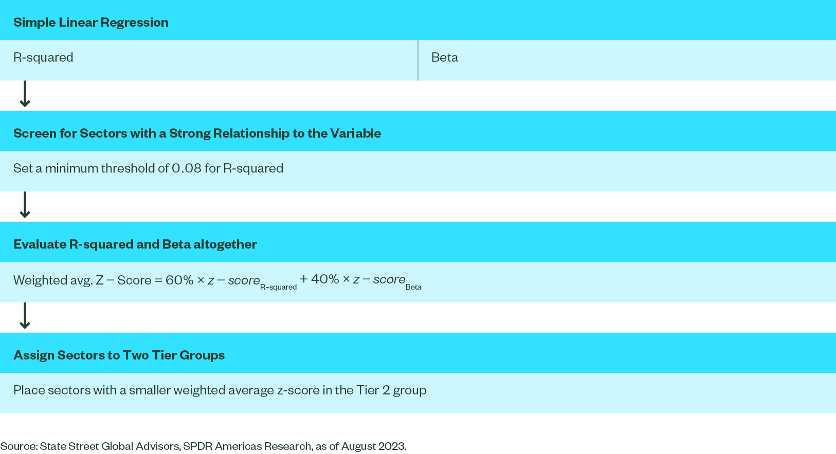
A simple linear regression model evaluates:
- The strength of the relationship between sectors’ relative returns and specific macroeconomic variables, as measured by R-squared of the regression model.
- The significance of the impact, as measured by the coefficient of the variable, commonly known as beta.
Focusing on relative returns removes effects of market beta on sector performance and transforms the time series to a stationary data set for regression analysis. We also tested the significance of coefficient (t-test), autocorrelation, and normality of the error distribution from the regression model to ensure coefficient estimates are reliable and statistically different from zero.
Defining Strong Relationships Between Sectors and Macro Variables
With so many unmeasured variables that can impact sector performance and all the noise in macroeconomic data, identifying a single macroeconomic variable that can explain even a small portion of sector performance gives investors valuable information.
To uncover that information edge, we set a minimum threshold of 0.08 for R-squared to screen for sectors with a strong relationship to the variable. What that means is if the macroeconomic variable can explain more than 8% of the variance of sector returns, we consider the relationship between the variable and the sector to be strong.
Evaluating the Magnitude of Impact
The magnitude of the impact of macroeconomic variables, measured by beta, is also worth review. For example, both Metals & Mining and Capital Markets industries have exhibited strong negative correlation with the US dollar (USD). However, beta for the Metals & Mining is much greater than for the Capital Markets industries. In other words, a 1% depreciation of the USD may provide more tailwinds for Metals & Mining than for Capital Markets.
To evaluate R-squared and beta altogether, we calculate weighted average z-score of R-squared and beta for sectors that passed the previous screen under each macroeconomic variable. We gave R-squared a greater weight (60%) in the z-score, since the strength of the relationship is a prerequisite to consider sectors for positioning against macroeconomic variables.
What is a z-score? Z-score measures how many standard deviations an element is above or below the population mean. A sector z-score can be calculated from the following formula. z = (X - μ)/σ, where X is the sector value of the metrics, μ is the mean of 11 sector values for a certain metric, and σ is the standard deviation of the value of 11 sectors.
There is one caveat to the sector beta estimates, which led us to group sectors that passed the initial screen into two tiers based on the weighted average z-score, instead of directly ranking them. While the beta for some sectors is statistically different from zero, their 95% confidence intervals — or the range of the beta that covers the true value 95% of the time — are quite wide and sometimes overlap with each other (see Appendix II). We placed sectors with a smaller weighted average z-score in the Tier 2 group.
See Appendix II for R-squared, beta, and z-scores of listed sectors. Sectors identified as having a strong relationship to macro variables are listed in the table below.
Figure 3: Sectors With Strong Relationships to Macro Variables
| 10-Year Yield | 10-Year Breakeven | USD | Oil | ||
|---|---|---|---|---|---|
| Positive | Tier 1 | Insurance^ Financials Banks Regional Banks |
Oil & Gas Equipment & Services Metals & Mining |
Cons. Staples |
Oil & Gas Equipment & Services
|
| Tier 2 | Oil & Gas Exploration & Production Industrials^ |
Oil & Gas Exploration & Production* |
Metals & Mining | ||
| Negative | Tier 1 | Communication Services | Cons. Staples Health Care |
Metals & Mining Materials Oil & Gas Equipment & Services |
Health Care Cons. Staples Utilities*^ |
| Tier 2 | Tech^ | Capital Markets* |
Source: State Street Global Advisors, SPDR Americas Research, as of December 2022. Past performance is not a reliable indicator of future performance. *R-squared is greater than 0.08 and less than 0.1. ^Sectors that didn’t show strong correlation for the sample periods when the macroeconomic variable had a greater than one standard deviation move.
Macro Variables’ Impact on Sectors Aligns with Intuition
Our findings on how macro variables impact sectors are generally in line with economic intuition.
- Commodities related sectors, such as Oil & Gas industries and Metals & Mining are most sensitive to oil prices and the USD, since the two variables directly impact commodity prices. These sectors are also positively correlated to inflation expectations, as higher commodity prices tend to lift inflation expectations and increase the sectors’ profits.
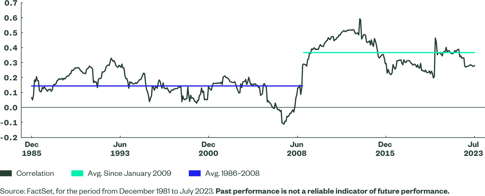
- Cyclical industries like Financials and Energy tend to move with 10-year yields, as higher 10-year yields generally point to strength in economic growth. Energy’s high sensitivity to 10-year yields is more likely driven by the high correlation between 10-year yields and oil prices since 2009, as shown in the chart below.
- Communication Services and Tech have negative correlation to 10-year yields that can be explained by their growth-oriented, long-duration profile, as higher risk-free rates weigh more on growth stock valuations.
- Defensive sectors like Health Care and Consumer Staples tend to outperform amid lower oil prices, declining inflation expectations, and a stronger USD, resulting from a weaker economic outlook and risk-off sentiment.
Figure 4: 5-Year Rolling Correlation of Oil Monthly Return and 10-Year Yield Changes
Gauging Sector Sensitivity to Macroeconomic Shocks
To find out whether relationships between sectors and macroeconomic variables would be strengthened or weakened by dramatic changes in variables, we divided the data sample into two groups based on the macroeconomic variable’s deviation from its historical average. If the variable is more than one standard deviation away from the average, we consider the change to be dramatic.
The table below shows the R-squared of the simple linear regression between sectors and each macroeconomic variable in the two data groups. Most sectors show stronger correlation to the variable when there are more dramatic changes to the variable.
On the other hand, when changes are within one standard deviation, R-squared of all sectors (except for Energy industries in relation to oil prices) declined below the minimum threshold of 0.08. This indicates an insignificant linear relationship when movements in macroeconomic variables are less significant.
Figure 5: Sector Sensitivity During Macroeconomic Shocks
| Between 1stdv R Sqr |
Greater than 1 Stdv R Sqr |
||
|---|---|---|---|
| 10-Year Breakeven Monthly Level Change Since 7/1/2003 |
Oil & Gas Equipment & Services | 0.054 | 0.285 |
| Metals and Mining | 0.03 | 0.379 | |
| Oil & Gas Exploration & Production | 0.06 | 0.12 | |
| Health Care | 0.033 | 0.171 | |
| Cons. Staples | 0.018 | 0.214 | |
| USD Weekly Return Since 1/1/2000 |
Metals and Mining | 0.047 | 0.496 |
| Cons. Staples | 0.011 | 0.363 | |
| Materials | 0.028 | 0.283 | |
| Oil & Gas Equipment & Services | 0.052 | 0.343 | |
| Capital Markets | 0 | 0.393 | |
| Oil Weekly Return Since 1/1/2000 |
Oil & Gas Equipment & Services | 0.196 | 0.447 |
| Oil & Gas Exploration & Production | 0.184 | 0.459 | |
| Energy | 0.143 | 0.402 | |
| Metals and Mining | 0.047 | 0.273 | |
| Health Care | 0.028 | 0.109 | |
| Cons. Staples | 0.029 | 0.108 | |
| Utilities | 0.005 | 0.028 | |
| 10-Year Treasury Yield Monthly Level Change Since 7/1/2003 |
Insurance | 0.001 | 0.001 |
| Oil & Gas Equipment & Services | 0.024 | 0.19 | |
| Financials | 0.012 | 0.113 | |
| Energy | 0.019 | 0.123 | |
| Regional Banks | 0.03 | 0.108 | |
| Bank | 0.04 | 0.228 | |
| Oil & Gas Exploration & Production | 0.038 | 0.141 | |
| Comm Svs. | 0.041 | 0.117 | |
| Industrials | 0.003 | 0.05 | |
| Tech. | 0.002 | 0 |
Source: State Street Global Advisors, SPDR Americas Research, as of December 2022. R-squared greater than 0.08 is highlighted in green. Past performance is not a reliable indicator of future performance.
Charting the Yield Curve’s Impact on Sectors
The slope of the yield curve has been closely watched by investors and monetary policymakers to project the future state of the economy. Monetary policy has a significant influence on the yield curve spread, economic activity, and short-term equity market performance.
Expectations of future inflation and monetary policy contained in the yield curve spread also influence forecasts for economic growth, which in turn influence stock prices. The yield spread of 10- and 2-year Treasurys is used as a proxy for the slope of the yield curve. Widening yield spreads indicate a steepening yield curve, while tightening spreads indicate a flattening yield curve.
We first conducted the Chi Square Test for Independence to determine if there is a significant relationship between the types of yield curve change (steepening or flattening) and sector performance (under/outperform the market). This helped us narrow our focus for further analyzing impact down to these nine sectors: Banks, Regional Banks, Capital Markets, Oil & Gas Equipment & Services, Software & Services, Consumer Staples, Financials, Real Estate, and Utilities.
We broke down the yield curve changes into six categories based on the direction and relative level of changes in 10-year and 2-year yields and created five dummy variables X1 ~ X5 = (0,1) to represent each type of yield curve in multiple linear regression analysis, as shown in Figure 6.
The intercept of the regression model (β0) is interpreted as the average relative return when the yield curve is bear steepening. β0 + β1 , β0 + β2, …… β0 + β5 are the mean estimate of relative returns given other five types of curve changes.
Figure 6: Yield Curve Multiple Regression Model and Types of Yield Curve Change
Sector Relative Return= β₀+ β₁×X₁+β₂×X₂+β₃×X₃+β₄×X₄+β₅×X₅
| Yield Curve Change | Definition | Variables and Coefficient | Mean Estimate of Relative Return | No. of Months in the Data Sample (Since July 2003) |
|---|---|---|---|---|
| Bear Steepen | 10-year yield increase > 2-year yield increase | Intercept, β0 | β0 | 52 |
| Bear Flatten | 10-year yield increase < 2-year yield increase | X1, β1 | β 0 + β1 | 49 |
| Bull Steepen | 10-year yield decrease < 2-year yield decrease | X2, β2 | β 0 + β2 | 22 |
| Bull Flatten | 10-year yield decrease > 2-year yield decrease | X3, β3 | β 0 + β3 | 72 |
| Twist Flatten | 10-year yield decrease, 2-year yield increase | X4, β4 | β 0 + β4 | 20 |
| Twist Steepen | 10-year yield increase, 2-year yield decrease | X5, β5 | β 0 + β5 | 19 |
Source: State Street Global Advisors, SPDR Americas Research, as of December 2022. Past performance is not a reliable indicator of future performance.
Linear regression models for Banks, Regional Banks, Real Estate, and Utilities show an adjusted R-squared greater than 0.08, indicating yield curve movements have significant explanation power for these sectors’ returns.
The table below shows the mean estimate of relative returns for various yield curve changes. The estimates that passed the significance test of coefficient (t-test) are highlighted in green. However, estimates for Bull Steepen, Twist Flatten, and Twist Steepen types of the yield curve should be taken with a grain of salt, since there are only about 20 observations under each of those scenarios in our data sample.
Figure 7: Estimated Mean of Relative Sector Returns (%)
| Bear Flatten | Bear Steepen | Bull Flatten | Bull Steepen | Twist Flatten | Twist Steepen | |
|---|---|---|---|---|---|---|
| Banks | -0.404 | 1.846 | -1.914 | 0.686 | -0.574 | -1.244 |
| Regional Banks | -0.385 | 1.955 | -1.785 | 0.465 | 0.235 | -1.125 |
| Real Estate | -0.463 | -2.09 | 1.783 | -0.036 | -1.871 | -0.369 |
| Utilities | -0.125 | -2.2 | 1.278 | 0.158 | -1.597 | -0.417 |
Source: State Street Global Advisors, SPDR Americas Research, as of December 2022. Past performance is not a reliable indicator of future performance. Green shades highlight the estimates that passed the significance test of coefficient (t-test).
This analysis of the yield curve’s impact on sectors is consistent with expectations:
- Banks: Since banks borrow at short-term rates and lend at long-term rates, a steepening yield curve generally provides tailwinds for banks’ profits, while a flattening curve means headwinds. Under the bear steepening scenario, higher rates on both the long and short end of the curve indicate that tightening monetary policies are not expected to hinder positive growth prospects, which further support demand for credits and bank revenue growth.
- Utilities and Real Estate: Low Treasury yields also make Utilities’ and Real Estate’s high dividend income more attractive to investors. Lower yields also generally point to a weaker economic growth outlook and risk-off market sentiment, which favor high dividend defensive stocks in Utilities and Real Estate.
Figure 8: Summary of Yield Curve’s Impact on Sectors
| Bear Flatten (10-year yield increase < 2-year yield increase) | Bear Steepen (10-year yield increase > 2-year yield increase) | Bull Flatten (10-year yield decrease > 2-year yield decrease) | |
| Positive | Bank; Regional Bank | Real Estate; Utilities | |
| Negative | Bank; Regional Bank; Real Estate; Utilities | Real Estate; Utilities | Bank; Regional Bank |
Source: State Street Global Advisors, SPDR Americas Research, as of December 2022. Past performance is not a reliable indicator of future performance.
Sector Performance Influenced by Additional Variables
While this research focused on the impacts of a short list of macroeconomic variables, we acknowledge that sector performance is influenced by many variables beyond the ones analyzed. This includes other economic variables, industry-specific secular trends, valuations, monetary policy, and short-term market sentiment.
Given the complexity and interactive nature of economic variables, it’s difficult both to anticipate which variables will drive sector returns and also to judge whether the macro expectations are priced in. Rather than predict sector performance using these variables, this research helps investors understand which sector relationships with macroeconomic variables appear most meaningful over a nearly 20-year period.
Due to the limitation of linear regression models, this research identifies only sectors that have strong linear relationships with the macro variables. Sectors may have more complicated relationships that require a non-linear model to formulate. Of course, a more complicated non-linear approach would come at the expense of an easily understood and interpretable model.
Rather than use this research alone to predict sector performance or provide sector rotation trading signals, investors should use it together with sector fundamental analysis and our sector business cycle framework, to evaluate the merits of investing in certain sectors under specific economic conditions.