Gain a Tax-efficient Edge and Broad Market Beta with Sectors
Investors looking to improve the after-tax returns of their US equity portfolios may want to consider a sector replication strategy. Disaggregating the market and investing in the 11 GICS sectors, with their year-over-year (YoY) differences in performance, can offer more tax-loss harvesting opportunities than just a single broad US equity exposure.
And when those GICS sectors are combined, and held at their respective market-cap weights, they can help replicate that broad beta exposure — seeking to avoid market drift while targeting increased tax-loss harvesting opportunities.
Tax-loss harvesting means selling investments in taxable accounts that have lost value to offset capital gains elsewhere in your portfolio and help reduce taxes owed. When you sell a position that has lost value:
- The loss offsets capital gains from selling securities at a profit during the year, as well as annual capital gain distributions of mutual funds.
- If capital losses exceed gains at year-end (or if there are no gains), losses can offset up to $3,000 in non-investment income, which is often taxed at a higher rate than capital gains.
- You can carry forward losses above $3,000 to offset capital gains and ordinary income over your lifetime.
Notably, the Internal Revenue Service’s Wash-Sale Rule prohibits claiming a loss on the sale of an investment if the same or “substantially identical” investment is purchased either 30 days before or after the sale date. Instead, a “tax swap” can serve as a placeholder to maintain exposure to the asset class for 30 days. After 30 days, you can decide whether to switch back to the original holding.
Sector Dispersion Means More Harvesting Opportunities
Why choose sectors to pursue a more tax-efficient portfolio? The GICS sectors historically have had a wide dispersion of returns.
The average dispersion of returns across sectors, based on trailing 1-year returns, is 44% (Figure 1). One-month, three-month, and six-month return dispersion is, on average, 29%, 20%, and 11%, respectively.1 This compares to 6%, 4%, and 2% for Growth and Value style exposures over those same time frames,2 suggesting that a sector replication strategy could be more valuable than a stylistic one when seeking to harness dispersion trends.
These differentiated sector return trends hold over different time frames as well as co-movement metrics too. Sectors’ 90-day average pairwise correlation of 59% compares to styles’ 92%3 — and the lack of co-movement across sectors varies based on market regimes (Figure 2). Wide dispersion and non-stationary correlations indicate sector returns can be meaningfully different, a potential benefit when seeking to harvest losses frequently across multiple market cycles.
Quantifying Tax-Loss Harvesting Opportunities
Tax-loss harvesting opportunities obviously depend on when investors buy a fund, as that establishes the cost basis for tax purposes. Rebalancing frequency also could impact tax lots.
To quantify tax-loss harvesting opportunities beyond identifying a wide dispersion of returns and low pairwise correlations, we calculated US sectors' return path from 1989 to 2023 to find sectors with negative trailing 1-year returns and negative trailing 1-year returns, when the S&P 500® itself had a positive return over the same time frame.
Calculated monthly, we found that, on average:
- At least three sectors had a negative 1-year return at once.
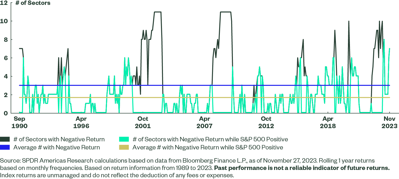
- During sizeable market downturns, all sectors tended to be in the red (Figure 3).
- All sectors weren’t up when the market was up. Roughly two sectors, on average, were down while the market was up over the prior year.
In sum, over the 399 months analyzed, at least one sector had a negative return in 288 of those months, or 72% of the time. Expanding the frequency to daily increased the probability to 73% of the time (6,315 over 8,651 days) a sector was at a loss over the most recent one-year period.
More specifically, if you had implemented a sector replication strategy at the start of 2022, you could have harvested Tech sector positions seven times and Communication Services sector ten times.4 Only one sector, Energy, didn’t offer any harvesting opportunities.5
Figure 3: Sectors Can Be Down While the Market Is Up
Creating a Broad Market Exposure with Sectors
To construct a disaggregated market-cap weighted exposure, you need a reference market and associated weights.
We used the S&P 500 Index and its historical sector weights on a monthly, quarterly, and semi-annual basis going back to 1998, which captures numerous market cycles and systemic events, from the dot-com bubble to the Global Financial Crisis and COVID-19 pandemic. We used the same periods as the assumed rebalancing time frames for the sector portfolio blend.
The frequency of rebalancing is important.
More frequent rebalancing means less market drift, but also potentially higher transaction costs that can cut into returns. While quarterly rebalancing aligns with the S&P 500 Index, there is no definitive “best” rebalancing period. In a real-world setting, rebalancing could be market driven, based on a sector position trading at a loss.
You might ask: Why not buy and hold the sectors at their respective weights in 1998 and never rebalance? After all, if the sectors themselves are market-cap weighted, shouldn’t the composure change as it would in the broad S&P 500, so the sector weights at all times match the S&P 500 based on the broad sector’s own return path? There are no sector constraints in the S&P 500 after all.
Importantly, this approach would not have captured the restructuring of the GICS map in 2016 and 2018 when new sectors were created. It also would not reflect corporate actions or additions and deletions to the S&P 500 that change the sector weights over time (e.g., if a Technology firm is removed from the S&P 500 and a Financial firm is added, the sector weights change).
Replicating Broad Beta with Sectors
While the probability of having more opportunities to harvest losses and reduce taxes supports using sectors and regularly rebalancing to mirror the market, investors don’t want to sacrifice returns.
To that end, we ran a blended portfolio of sector exposures with the historical weights and assumed rebalancing periods from 1998 to 2023 versus the S&P 500 (Figure 4). Across all three rebalancing types, the sector returns mirrored the return on the S&P 500 Index quite closely. Both the correlation and beta sensitivity of the portfolios were 16 and the volatility profiles were also similar. For example, on the monthly rebalanced sector S&P 500 portfolio, the standard deviation of returns was 14.9% versus 15.3% for the S&P 500 Index over this 25-year time frame.7
Figure 4: Sector Returns Closely Mirror S&P 500 (December 1998 to December 2023)
| Sector – Monthly | Sector - Quarterly | Sector - Semi-Annual | S&P 500 | |
|---|---|---|---|---|
| Cumulative Return | 306% | 301% | 294% | 272% |
| Annualized Return | 5.80% | 5.70% | 5.60% | 5.40% |
Source: SPDR Americas Research calculations based on data from Bloomberg Finance as of December 4, 2023. Based on return information from 12/1998 to 12/2023. Past performance is not a reliable indicator of future performance. Index returns are unmanaged and do not reflect the deduction of any fees or expenses. Index returns are price returns and do not reflect all items of income, gain and loss and the reinvestment of dividends and other income.
Of course, annualized figures can overshadow the inter-return period dispersion, based on slippage resulting from slight weighting differences. Examining both monthly return variances and rolling return periods can determine if the deviations are outsized. After all, dispersion can be friend and foe with this process.
But the median monthly return difference for the monthly rebalanced portfolio to the S&P 500 Index was just -0.01%. And when there were larger variances, particularly during a crisis or market event, they tended to mean-revert month-over-month (Figure 5).
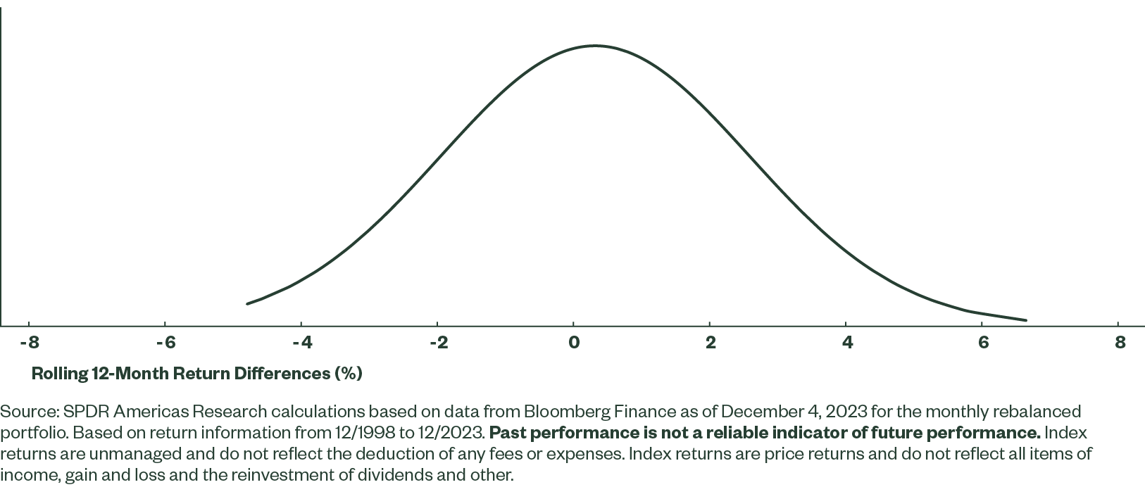
Additionally, the average 12-month difference in return was just 0.3% (median 0.2%) over 289 analyzed rolling 12-month periods. Here, too, differences tended to mean revert upon the next rebalance. More in-depth statistical analysis indicates the return differences largely follow a normal distribution pattern (2% standard deviation) with a slight positive right skew of 0.1 and minor negative kurtosis (-0.36) (Figure 6). A negative kurtosis implies a distribution with less extreme possible data values (i.e., there are no massive outliers of these return differentials).
Figure 6: Sectors’ Rolling 12-Month Return Differences Reflect a Normal Distribution Pattern
Why Choose Sector ETFs
Investors looking to gain an edge, without taking on substantial additional risk or slippage in their US equity portfolios, may want to consider the relative performance benefits of a sector replication strategy. When regularly rebalanced, a blended sector portfolio may offer more opportunities to harvest tax losses, potentially improving after-tax performance.
Using sector ETFs with their liquidity, market access, and transparency makes it easy to compare market coverage and underlying stock weights with the S&P 500 Index and implement a sector replication strategy.
Check out our ETF education hub to learn more about topics like ETF due diligence, trade optimization, and portfolio construction. Or for more on sector investing trends and approaches, explore our latest sector insights.