Putting Investment Decisions Into Context

While it’s certainly prudent for investors to examine cyclical indicators that provide context on how smooth or rocky the environment is for fixed income investing, the approach to doing so and the data used by investment managers can vary widely. In this piece, we describe an approach in which we determine which market return cycle is occurring (i.e., repair, decline, recovery or expansion), and then use that information to project future returns and allocate risk to different fixed income segments. This cycle-aware approach focuses on cyclical indicators whose variance tends to result in differentiated future returns. As part of the process, we also analyse spread data to help decide whether markets are cheap or expensive based on historical data for each phase of the cycle.

The Cycle as a Context Provider

Investors have a multitude of ways to get context for their investment decisions. Frequently, a story or narrative (that is not necessarily data-driven) becomes the basis for how investors get a sense of the market. These narratives, combined with behavioural biases that give more recent information a disproportionately high weight, ¹create an “inside view” that can lead to insufficient context.²

Research on the optimal approaches to decision making, highlights the importance of starting instead with an “outside view”—a broader set of similar market environments or “reference classes,” and historical data. The next step is to account for current specifics. Many investors instead go in the opposite order, taking current, recent information, and drawing broader conclusions. The commonality—or lack thereof—of past circumstances versus current can increase (or decrease) the importance of starting with a wider view.

One way to get context via an outside view, is to look closely at inputs whose variance tends to result in differentiated future returns. This may seem obvious, but most cyclical indicators tend to either try to predict recession probabilities or track the economic cycle. A more direct and useful exercise would be to track data whose level and recent change has historically identified differentiated quadrants of both risk and return. These quadrants can be thought of in the traditional expansion, decline, recovery, and repair phases. For example, if the data is above average and still improving, that would be an expansion phase. If the data is above average and disimproving, that would be decline.

Using the Cyclical Indicators to Forecast Returns

Inputs that are most useful in tracking this return cycle tend to:

• Provide a sense of the monetary policy stance (for example, the yield curve).
• Indicate the level of debt in the economy and the willingness of consumers and corporations to take on more leverage.
• Indicate the likely stage of the economic cycle (for example, jobless claims).

Once identified, historical future performance and risk can be summarised for each sector in each phase. For example, using an average of 9 indicators that have typically led the return cycle would suggest that after spending all of 2022 and up to April 2023 in the expansion phase, we have recently moved into the decline phase. Using data from the last 30 years, Figure 1 shows the historical next 12 months performance (percent) for each fixed income sector in each phase.

Insights on the Current Phase

By examining how each sector performed in the period following each regime, we can summarize a few thoughts on the current phase:

• Typically, the move from expansion to decline favours duration, and especially curve steepening positions, over spread exposure. Given the bull market in bonds that lasted for the bulk of our 30-year data set, duration exposure implies positive 12-month-forward returns in all regimes. So more appropriately for duration, when looking in relative rather than in absolute terms, the expansion phase is typically the weakest for duration returns, with returns in the decline phase being twice those in expansion. 
• Partly explaining the performance of duration and curve steepening positions is that inflation tends to peak in the late expansion and early decline phases. From 1987 to 2023 US inflation averaged 3% in decline, 2.6% in expansion and 2.1% in the other phases. 
• High Yield and Investment grade forward excess returns have not only been negative in the decline phase, but the volatility of those returns has been more than double of that seen in the expansion phase. So typically less reward, with more risk for this spread exposure, as the cycle matures.

The Valuation Overlay

Armed with forward data on how each fixed income sector has typically traded in the 12 months following each regime, we can go a step further and look at how markets are currently priced, relative to history, based on the regime we are in.
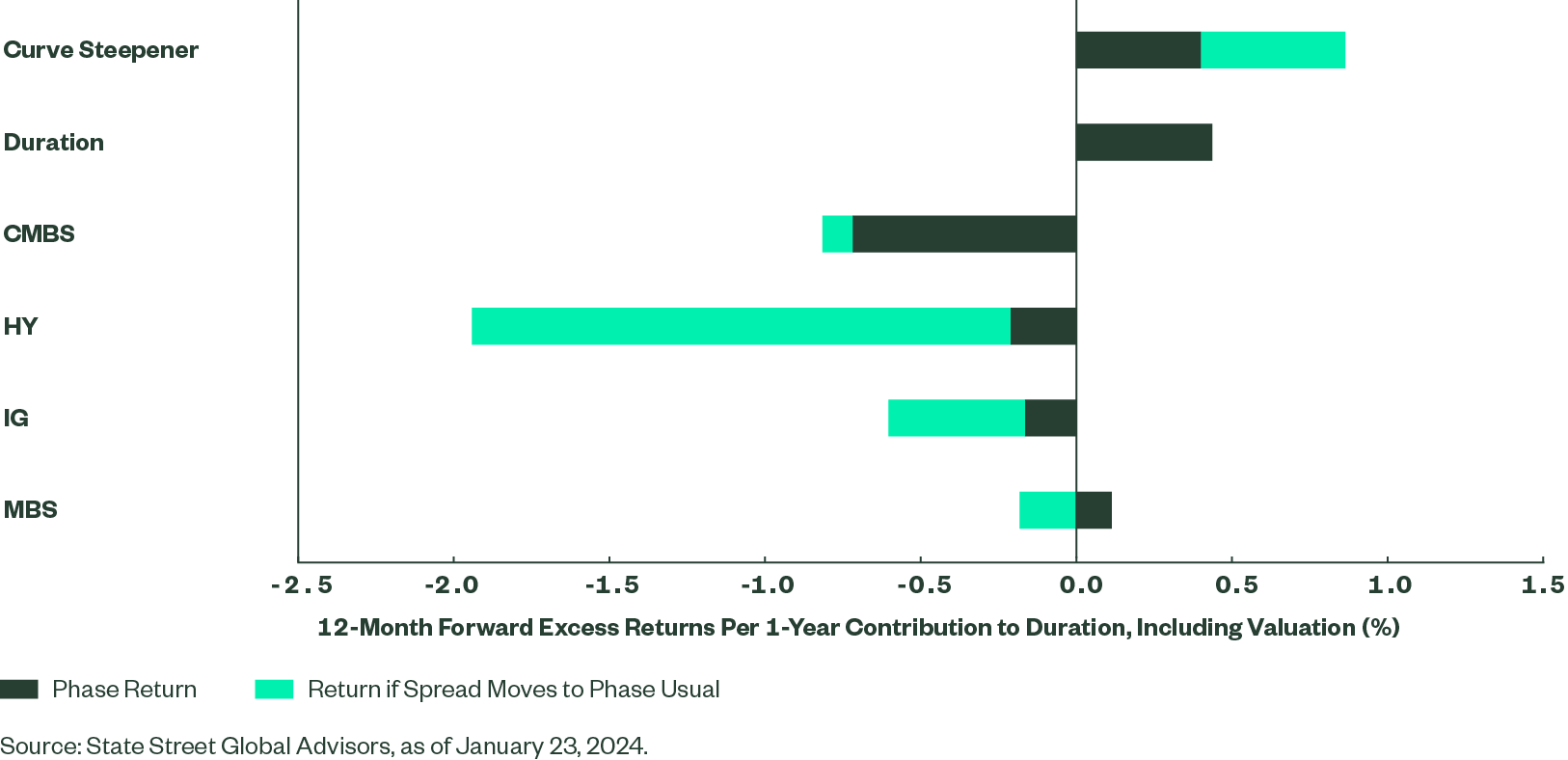
For example, Figure 1 shows that investment grade credit typically had an excess return of -17 basis points (bps) in the decline phase over the next 12 months per unit of duration; but, what if current spreads implied even lower excess returns? One possibility is that spreads could “mean revert” and widen to the usual phase average. This would negatively impact returns beyond what’s implied by the cycle alone (Figure 2). See the general formula below:

Expected Return Based on Historical Data for the Regime + Potential Change in Return Based on Mean Reversion of Spreads * % of reversion expected = Valuation-Adjusted Expected Return

Cycle-Aware Investing in Practice

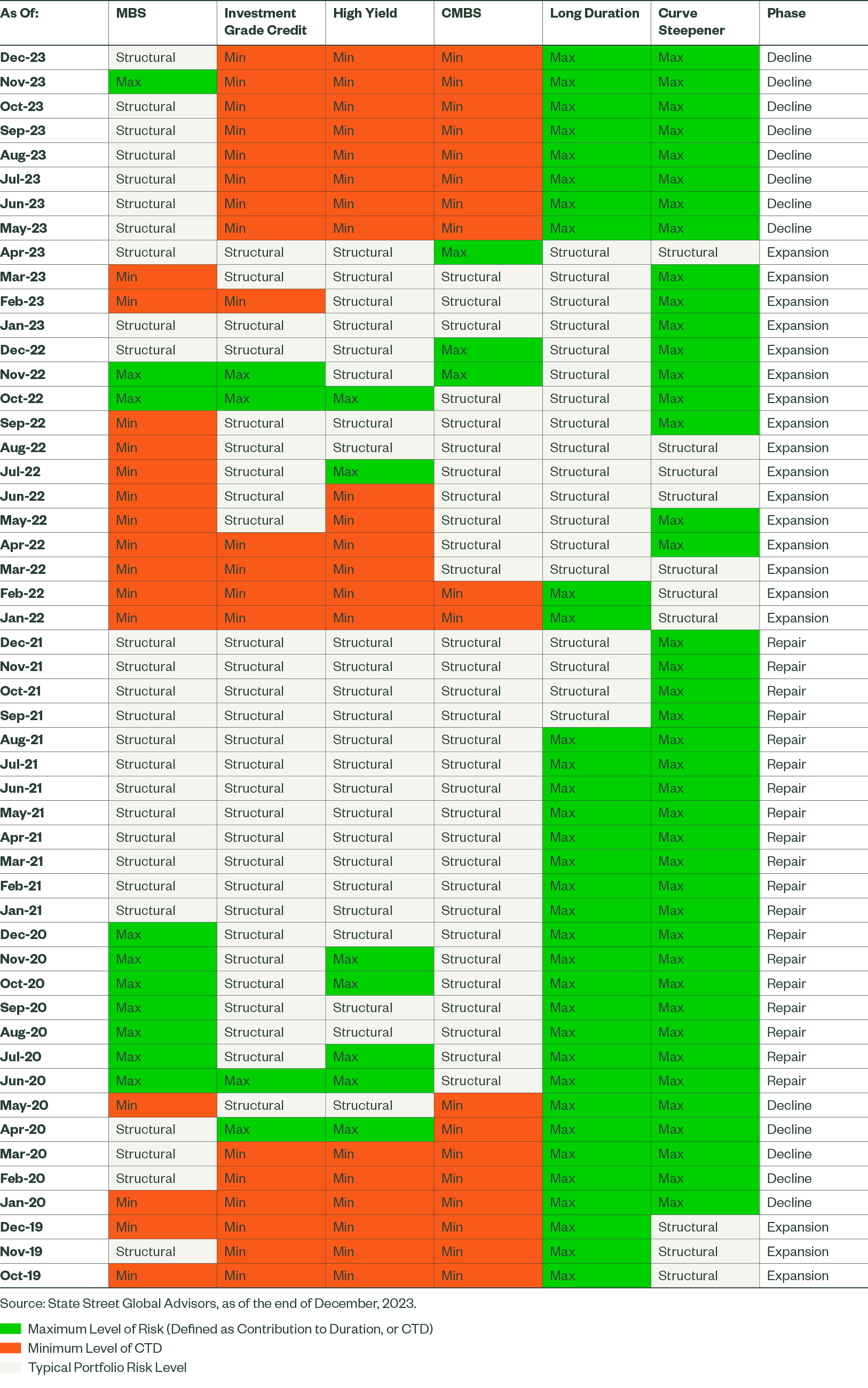
A more systematic approach taking valuations into account can easily be imagined. As part of the State Street Global Advisors Active Fixed Income team’s efforts to evaluate our cycle-aware investment process, we looked at historical data and calculated what a rules-based framework would have suggested once both cycle, risk, and valuations were taken into account (i.e. a valuation-adjusted sharpe ratio). The level of future returns for each fixed income sector in each phase, adjusted for valuations and risk, was used to calculate a suggested risk stance for each sector. Recent results are shown in Figure 3. This table shows that Integrating the Cycle Backdrop with Market Pricing Data Allows Us to Calculate a Valuation-Adjusted Sharpe Ratio, and suggested risk allocation for each segment.³

From the Outside to the Inside View

This approach shows how market segments performed when data that is usually relevant to that performance, was in a similar place to todays. We can then take valuation differences into account, but we also need to integrate the specifics of the day that may alter the historical experience.

At a minimum investors should question both the relevance of the data, and the authorities likely reaction to changes to it, relative to their reaction in the past. As an example; the US entered the pandemic as an outlier with regards to not having an official avenue to purchase corporate bonds. The Bank of England, European Central bank, and Bank of Japan all had well established corporate buying programmes as part of their quantitative easing arsenal. While the cyclical framework would have suggested that valuation adjusted spreads had become attractive, it was this specific question of when a corporate buying programme would be introduced that would prove decisive in timing credit spread exposure in this period. At the moment, investors need to decide if there is information specific to today, like the ability of the US authorities to buy corporate bonds if required or slower transmission of monetary policy, that warrants credit spreads trading inside what would be usual for not only a decline phase, but also a typical expansion phase.

More generally, over the past 20 years, a starting point of smaller central bank balance sheets, reduced government debt levels, alongside lower inflation than recently experienced have allowed aggressive policy responses when risk aversion has spiked in the markets. This backdrop rewarded a “buy the dip” mentality (i.e., taking advantage when spreads were wide versus historical averages for the cycle) that assumed a relatively quick mean reversion of valuations. Going forward, it may be more challenging for central banks to be extremely accommodative.

In conclusion, a cycle-aware approach can be a useful starting point for determining the appropriate level of risk taking in each segment, especially once then weighed against any unique features of the current environment.